2 The Generate Pipeline

2.1 Generating Stimuli

One of the most noteworthy features of LexOPS is that it can generate controlled stimuli for any possible factorial design. This can be done in a pipeline using 3 main functions:

split_by()

to specify “splits” (independent variables) in the experimental design

control_for()

to specify variables that should be controlled for between conditions

generate()

to run the algorithm and generate the stimuli, using specified splits and controls

A Practical Example

Imagine we want to generate stimuli for a 2x2 factorial design in a Lexical Decision Task, examining whether a possible effect of bigram probability interacts with concreteness.

For this, we might decide we want a stimulus set with the following features:

Filtered such that at least 90% of people know each word, according to Brysbaert, Mandera, McCormick, and Keuleers (2019).
Two levels of Concreteness (abstract and concrete words) according to Brysbaert, Warriner and Kuperman (2014).
Two levels of Bigram Probability (low and high probability) based on SUBTLEX-UK (van Heuven, Mandera, Keuleers, & Brysbaert, 2014).
Controlled for word length (number of characters) exactly.
Controlled for word frequency within ±0.2 Zipf, according to according to SUBTLEX-UK (van Heuven, Mandera, Keuleers, & Brysbaert, 2014).
25 words for each of the generated conditions (100 stimuli in total).

We can use the following R code to generate a stimulus list like this with LexOPS:

library(LexOPS)

stim <- lexops |>
  subset(PK.Brysbaert >= 0.9) |>
  split_by(CNC.Brysbaert, 1:2 ~ 4:5) |>
  split_by(BG.SUBTLEX_UK, 0:0.003 ~ 0.009:0.013) |>
  control_for(Length, 0:0) |>
  control_for(Zipf.SUBTLEX_UK, -0.2:0.2) |>
  generate(n = 25)

Important notes on LexOPS (non-standard) syntax:

As in the tidyverse, variables in the dataframe can be referenced outside of quotation marks.
The : character is used in split_by() to specify numeric boundaries (e.g. 0.009:0.013 means any number from 0.009 to 0.013 is acceptable for this level of the variable), and in control_for() to specify tolerances (e.g. -0.2:0.2 means controls will be acceptable if within ±0.2 of the match null).
The ~ character is used in split_by() to specify different levels of an independent variable (e.g. 1.5:2.5 ~ 3.5:4.5 ~ 5.5:6.5 would specify three levels).

Output

Let’s have a closer look at the first 5 rows of stim, which contains the output from above:

item_nr	A1_B1	A1_B2	A2_B1	A2_B2	match_null
1	ahoy	sane	burp	bong	A2_B1
2	subtlety	reasoned	choirboy	minstrel	A1_B2
3	unsafe	regain	juggle	strand	A1_B2
4	dynamics	inferior	bagpipes	intruder	A2_B2
5	signify	rousing	crumpet	warthog	A2_B2

We can see that we have 4 conditions:

A1_B1 (abstract, low probability)
A1_B2 (abstract, high probability)
A2_B1 (concrete, low probability)
A2_B2 (concrete, high probability)

Each row of the dataframe is controlled for in terms of frequency and length. The match_null variable tells us which condition stimuli were matched relative to. For instance, we can see that in row 3, items are matched relative to the word “relent”. This means that all words for item_nr 3 are within ±0.2 Zipf of the Zipf value associated with the word “relent”. By default, LexOPS will select the match_null for each item pseudo-randomly, such that each condition will be used as a match null an equal number of times (match_null = "balanced"), or as close to this ideal as is possible (e.g. the number of items requested may not be divisible by the number of conditions). See this FAQ section for more information on match nulls.

2.2 Converting to Long Format

The table above shows the generated stimuli in wide format. This is a useful way to quickly view the stimuli and get a sense for what has been generated, but we often want to check our stimuli in more detail. The long_format() function is a quick way to convert stimuli generated in LexOPS into long format:

stim_long <- long_format(stim)

Now we have the same stimuli in long format, with their associated values. Here are the same first 5 matched items from earlier, but in long format:

item_nr	condition	match_null	string	Zipf.SUBTLEX_UK	Length	BG.SUBTLEX_UK	CNC.Brysbaert
1	A1_B1	A2_B1	ahoy	3.270924	4	0.0024671	2.00
1	A1_B2	A2_B1	sane	3.351834	4	0.0097561	1.79
1	A2_B1	A2_B1	burp	3.311686	4	0.0029034	4.34
1	A2_B2	A2_B1	bong	3.450084	4	0.0095689	4.27
2	A1_B1	A1_B2	subtlety	2.913220	8	0.0025943	1.54
2	A1_B2	A1_B2	reasoned	2.729160	8	0.0101181	1.64
2	A2_B1	A1_B2	choirboy	2.559059	8	0.0027849	4.56
2	A2_B2	A1_B2	minstrel	2.905251	8	0.0100126	4.11
3	A1_B1	A1_B2	unsafe	3.487426	6	0.0023499	1.89
3	A1_B2	A1_B2	regain	3.532060	6	0.0099835	1.79
3	A2_B1	A1_B2	juggle	3.365053	6	0.0024606	4.04
3	A2_B2	A1_B2	strand	3.478208	6	0.0099946	4.10
4	A1_B1	A2_B2	dynamics	3.281197	8	0.0019895	1.96
4	A1_B2	A2_B2	inferior	3.210284	8	0.0096549	1.70
4	A2_B1	A2_B2	bagpipes	3.162603	8	0.0028140	4.93
4	A2_B2	A2_B2	intruder	3.294526	8	0.0092513	4.14
5	A1_B1	A2_B2	signify	2.910580	7	0.0020770	1.73
5	A1_B2	A2_B2	rousing	3.109036	7	0.0119233	1.55
5	A2_B1	A2_B2	crumpet	2.848024	7	0.0023334	4.81
5	A2_B2	A2_B2	warthog	2.979037	7	0.0110464	5.00

Here we can see that indeed, the different conditions are within the boundaries we set, and that the variables used as controls are matched for items with the same item_nr.

2.3 Plotting the Design

While having data in long format is undoubtably useful, it’s not very efficient if you want to check what your stimuli look like in a quick glance (especially if your stimuli number in the thousands). What you probably want to do is create a plot to see how your stimuli differ between conditions and across matched items. Thankfully, LexOPS has a handy function to do exactly that:

plot_design(stim)

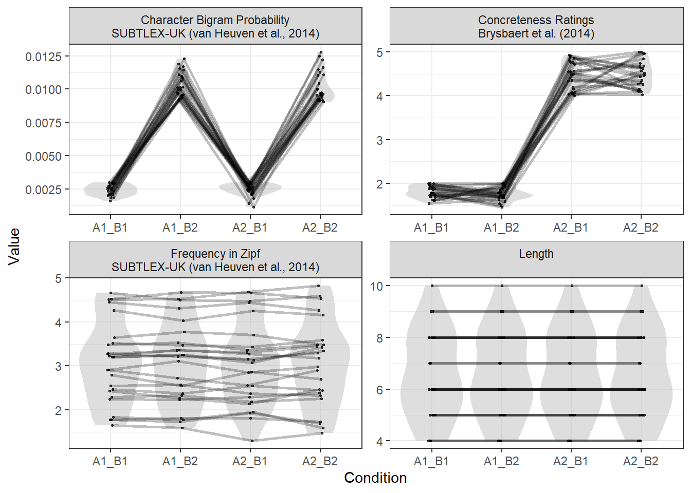
Figure 2.1: The results of the plot_design() function for the generated stimuli.

The distributions of all the numeric variables used as independent variables or controls are plotted for each condition (in a grey violin plot). The points depict the values of individual words, and points of the same colour (joined by lines) are matched items. As we’d expect, our example stimuli show the expected differences in Bigram Probability and Concreteness, while Frequency is matched closely, and Length is matched exactly.

2.4 Checking Representativeness

We can also visualise how representative our stimuli are. This shows the distributions of our generated stimuli on variables, relative to possible but unused candidates.

plot_sample(stim)

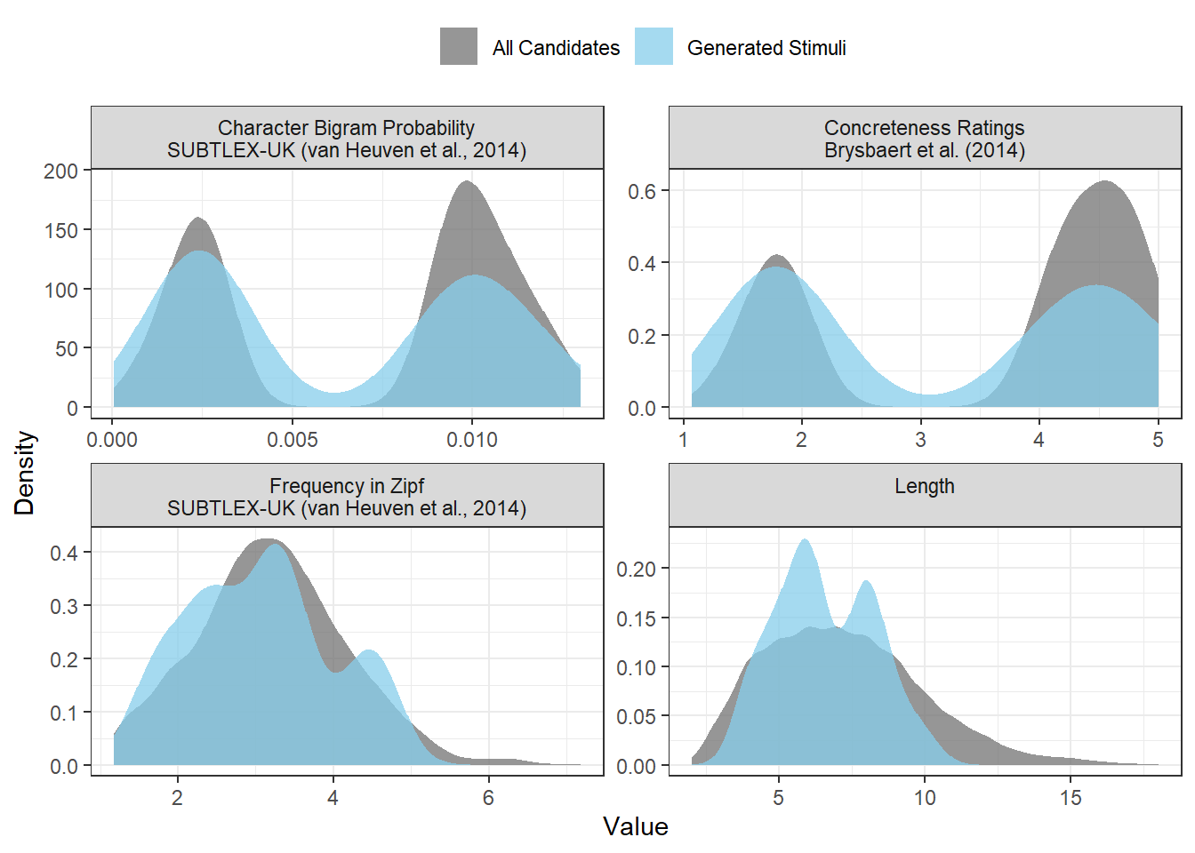
Figure 2.2: The results of the plot_sample() function for the generated stimuli.

2.5 Generating as Many as Possible

Let’s imagine that we’re not entirely sure how many stimuli we could generate using our design. It may be that the n = 25 we used earlier is considerably fewer than the number of stimuli we could generate with no problems. One way to test this is to have LexOPS generate as many stimuli as possible. We can do this by setting n = "all":

possible_stim <- LexOPS::lexops |>
  subset(PK.Brysbaert >= 0.9) |>
  split_by(CNC.Brysbaert, 1:2 ~ 4:5) |>
  split_by(BG.SUBTLEX_UK, 0:0.003 ~ 0.009:0.013) |>
  control_for(Length, 0:0) |>
  control_for(Zipf.SUBTLEX_UK, -0.2:0.2) |>
  generate(n = "all", match_null = "inclusive")

This is much slower, as LexOPS will continue trying to generate combinations of words that fit the specified characteristics until it has exhausted all the possibilities. Nevertheless, we actually generated 104 words generated per condition with the code above. This number is likely to change slightly each time we run the pipeline, as different combinations are randomly made from all the possible combinations. That said, it is a fairly good indication of the number of possible stimuli we could generate.

The 104 words we’ve managed to generate per condition here is quite a bit higher than the 25 we originally generated. Does this mean we should just request a larger stimulus list, such as n = 80, or even n = 100? Well, it depends. If we want as many stimuli as are possible, then it may make sense to just set n = "all", but often we only want to use as many stimuli as we need to find our effect. Also, if we use as many combinations as possible, experimenters who want to replicate our effect using a different set of stimuli will likely have fewer novel combinations available to them.

Note that when n = “all”, you will get a warning if you also keep the default match null setting, match_null = “balanced”. The reason for this is explained in this FAQ section.

2.6 Plotting Iterations

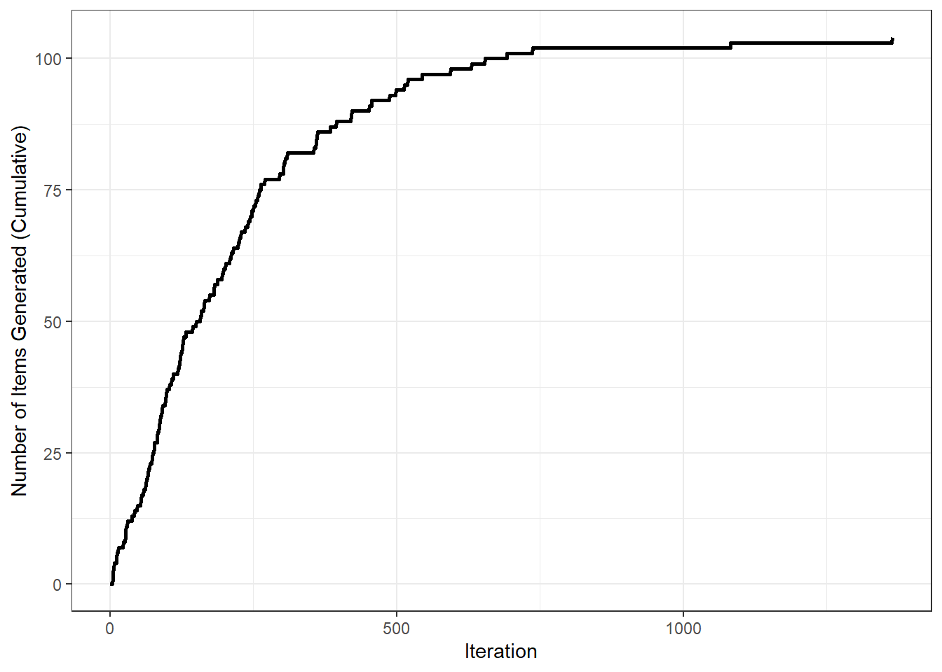
It is also possible to check how well LexOPS performed when generating stimuli by plotting the cumulative item generation by iterations. To do this, we can use the plot_iterations() function. As an example, let’s visualise the algorithm’s iterations when we generated as many stimuli as we could in the last section.

plot_iterations(possible_stim)

Figure 2.3: The cumulative number of items generated per iteration.

This shows a characteristic levelling-off; iterations become increasingly less likely to successfully generate items as the pool of possible combinations is gradually exhausted.

2.7 Custom Dataframes

While the LexOPS Dataset has lots of useful features for English, it isn’t exhaustive, and other languages do exist! The LexOPS functions will actually work with any dataframe, with words from any language. As an example, here’s how to generate a stimulus list of negative, neutral, and positive German words matched for length and frequency, based on the Leipzig Affective Norms for German (LANG) (Kanske & Kotz, 2010). Note that the set_options() function is used to tell LexOPS that our column containing the strings is "word", rather than the LexOPS default of "string".

library(readr)
LANG <- read_csv("kanske_kotz_2010.csv", locale=locale(encoding = "latin1"))

stim <- LANG |>
  set_options(id_col = "word") |>
  split_by(valence_mean, 1:3.5 ~ 4.75:5.25 ~ 6.5:9) |>
  control_for(number_of_letters, 0:0) |>
  control_for(frequency, -1:1) |>
  generate(20)

Here are the first five items generated for each condition:

item_nr	A1	A2	A3	match_null
1	hetze	blase	flirt	A2
2	bombe	stamm	komik	A3
3	pein	seil	kuss	A1
4	ärger	stein	humor	A3
5	terror	lehrer	gefühl	A1

For more detailed examples of how to use other datasets, the following vignettes might be useful:

Applications to Participant Selection: How you can use a dataset which has nothing to do with words.
Using Data from Custom Sources: How you can join the LexOPS dataset to other lists of word features.

Custom datasets can also be neatly integrated into the Shiny app. See this section for a example using custom variables in the shiny app.