About this post

I’ve decided to write a brief disclaimer about this post. Please don’t use this post for statistical advice. This post was mostly thinking out loud about a possible method of hypothesis testing, but in fact it just reinvents existing methods in a noisy way. Looking at the post again a few months later, I think it doesn’t tell us anything we can’t already get from existing methods. Another problem with this supposed method is that this defeats the whole point of a ROPE. The ROPE is a Region of Practical Equivalence, tying the hypothesis to some practically relevant interpretation. Arbitrarily deciding on regions with data-driven analyses isn’t really informative.

I’ve kept the post here because I know how annoying it is to follow a dead link.

If you’re interested in the problems with this post, this twitter thread might be useful: https://twitter.com/robustgar/status/1288810686752137217

The original (problematic) post

Hypothesis testing is a finicky business. The most common and traditional method, null-hypothesis significance testing (NHST) is actually pretty useful when all you want to know is whether your data is more extreme than you’d expect by chance, i.e. whether we have evidence against the null hypothesis. What about when your p-value is non-significant though? There’s a deep-seated temptation to incorrectly interpret this as evidence for the absence of an effect. In fact, this would be better described as a lack of evidence for the presence of an effect. This could indeed be because the null hypothesis is true, but it could also be because we just don’t have the data to support a conclusion either way. From a p-value, we have two possible situations:

• It’s significant: Evidence against the null hypothesis. Hurray, another paper in the bag!

• It’s non-significant: *shrug* who knows?

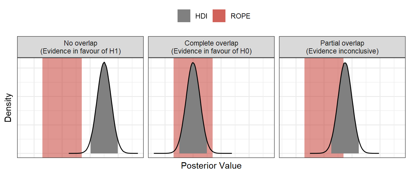
In Bayesian statistics, the Region of Practical Equivalence (ROPE) method is a fairly common approach to hypothesis testing which allows us to distinguish this “*shrug* who knows?” category into either inconclusive evidence, or evidence in favour of the null hypothesis. If it’s new to you, Kruschke (2018) gives a good introduction to the ROPE method. Using the ROPE method, we accept a null hypothesis if the credible interval of the relevant posterior distribution lies entirely within the ROPE. We reject a null hypothesis if the credible interval is entirely outside of the ROPE, and we remain undecided if there is partial overlap between the credible interval and the ROPE.

Maybe the most difficult part of using a ROPE to test hypotheses is deciding what the ROPE should be. This is not a problem exclusive to Bayesian statistics either (see the Smallest Effect Size of Interest of Equivalence Testing: Lakens et al., 2018). Some approaches focus on a cost-benefit analysis of the ROPE (with parallels to arguments about p-values), while in Psychological science, some suggest the ROPE should be defined by the smallest difference the subjects are able to detect or would judge as meaningful (Anvari & Lakens, 2019). Alternatively, you could derive a ROPE from previous studies and data, or build a computational model of the process you are looking at and decide via simulation on a difference you could expect by chance.

Sometimes none of these approaches are applicable, but you still want to test your hypotheses. Here, I’m going to outline a data-driven approach I’ve found useful before. The method consists of three basic steps:

1. Fit a model to the data you’ve collected

2. Randomly sample data to yield estimates you would observe under the null hypothesis

3. Treat the x% highest density interval of your samples derived from permutations as your ROPE

The data I’ll use is simulated below. There are three datasets, all generated with a simple linear model formula:

\[y_{i} = \beta0 + \beta1 + e_{i}\]

The datasets differ in terms of \(\beta1\) and \(e_i\):

• data1: \(\beta1=1\), \(e_i\sim N(\mu=0, \sigma=1)\)
• data2: \(\beta1=0.25\), \(e_i\sim N(\mu=0, \sigma=1)\)
• data3: \(\beta1=0.25\), \(e_i\sim N(\mu=0, \sigma=0.25)\)

library(tidyverse)
n_obs <- 50
intercept <- 0.5
betas <- c(1, 0.25, 0.25)
sigmas <- c(1, 1, 0.25)

data1 <- tibble(
  grp = rep(c(-0.5, 0.5), each=n_obs),
  y = rep(c(intercept, intercept+betas[1]), each=n_obs) + rnorm(n_obs*2, 0, sigmas[1])
)

data2 <- tibble(
  grp = rep(c(-0.5, 0.5), each=n_obs),
  y = rep(c(intercept, intercept+betas[2]), each=n_obs) + rnorm(n_obs*2, 0, sigmas[2])
)

data3 <- tibble(
  grp = rep(c(-0.5, 0.5), each=n_obs),
  y = rep(c(intercept, intercept+betas[3]), each=n_obs) + rnorm(n_obs*2, 0, sigmas[3])
)

1 - Fit the Model

Let’s build a simple model to each dataset, predicting y as a function of column grp. For simplicity, the default priors, model family, and sampling options will do.

library(brms)
m1 <- brm(y ~ grp, data = data1)
m2 <- brm(y ~ grp, data = data2)
m3 <- brm(y ~ grp, data = data3)

Here is a plot showing estimates, posterior distributions, and trace plots of chains for the effect of group in data1:

plot(m1, combo=c("areas", "trace"), pars="grp")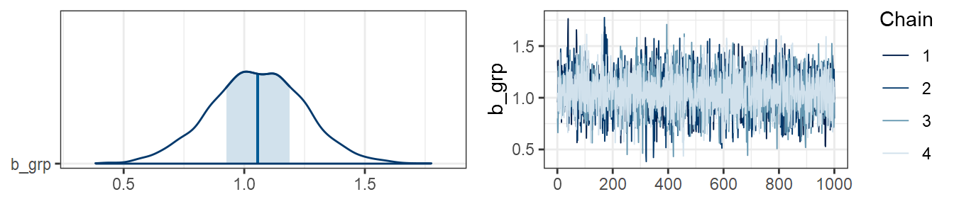

…and in data2:

plot(m2, combo=c("areas", "trace"), pars="grp")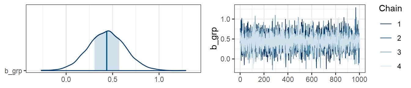

…and in data3:

plot(m3, combo=c("areas", "trace"), pars="grp")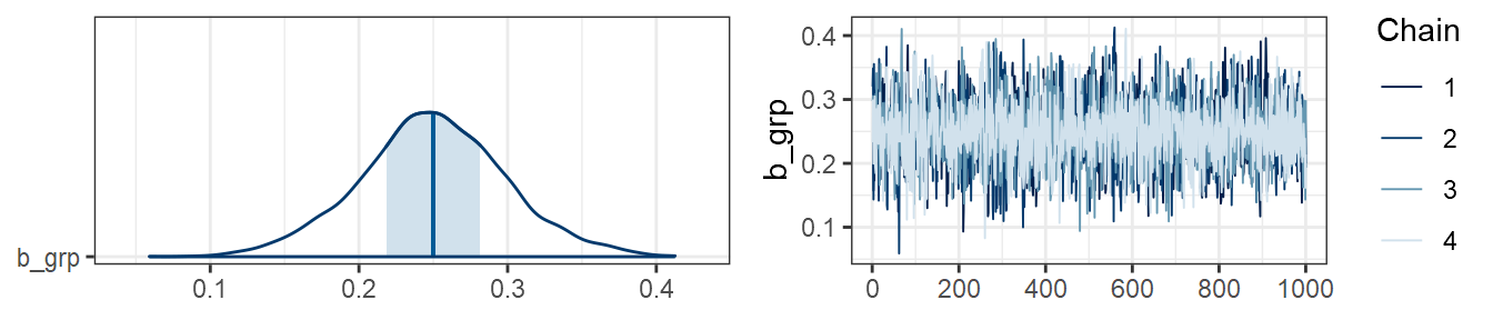

2 - Randomly Sample Data

The aim of this step is to get a distribution of observations we believe we could get if there were no effect of our predictor, grp. The method I’m going to suggest combines bootstrapping and permutations. On each iteration, we:

1. bootstrap by sampling our full dataset with replacement. The bootstrapping is done row-wise, so that each observation keeps the original information we have about it, and simulates variability in sampling.

2. permute the data by randomly sampling the values in the grp column without replacement. The permutations only shuffle values in the grp column, to simulate a situation in which the null hypothesis is true.

Here’s the function we’ll use for getting the bootstrapped, permuted data on each iteration:

bootstrap_permute <- function(dat) {
  dat %>%
    # 1. bootstrap: sample rows with replacement
    slice_sample(replace=TRUE, prop=1) %>%
    # 2. permute: sample grp without replacement
    mutate(grp = sample(grp))
}

We can run this 500 times to get a list of 500 datasets we could’ve observed under the null hypothesis, for each of data1, data2, and data3:

bsp_data1 <- replicate(500, bootstrap_permute(data1), simplify=FALSE)
bsp_data2 <- replicate(500, bootstrap_permute(data2), simplify=FALSE)
bsp_data3 <- replicate(500, bootstrap_permute(data3), simplify=FALSE)

Now we can fit a model for each dataset in bsp_data1, bsp_data2, and bsp_data3, using the same model settings as we used for the real data. To avoid having to recompile the model in C++, we can use the update() function to just change the data the models are fit to:

bsp_m1 <- lapply(bsp_data1, function(dat_i) update(m1, newdata=dat_i))
bsp_m2 <- lapply(bsp_data2, function(dat_i) update(m2, newdata=dat_i))
bsp_m3 <- lapply(bsp_data3, function(dat_i) update(m3, newdata=dat_i))

3 - Get the ROPE

If we collapse across the 500 models we got from bootstrapped permuted datasets, we get a sampling distribution of posterior samples under the null hypothesis. A way of visualising this is to overlay the distributions of posterior samples for the raw data with the samples from the bootstrapped permuted data. Here I highlight the 89% HDI credible intervals. The idea is that the 89% interval of our bootstrapped permutation samples can then serve as the data-driven ROPE.

library(ggdist)
library(ggridges)
library(ggstance)

Ms <- list(m1, m2, m3)
bsp_Ms <- list(bsp_m1, bsp_m2, bsp_m3)

res <- map_df(1:3, function(data_nr) {
  # get the true data's posterior samples
  post_long <- posterior_samples(Ms[[data_nr]]) %>%
    pivot_longer(c(b_Intercept, b_grp), names_to="param", values_to="value") %>%
    mutate(src = "True Posterior Samples")

  # get the posterior samples from all models fit to bootstrapped-permuted data
  bsp_post_long <- map_df(1:length(bsp_Ms[[data_nr]]), function(bsp_nr) {
    bsp_Ms[[data_nr]][[bsp_nr]] %>%
      posterior_samples() %>%
      select(b_Intercept, b_grp) %>%
      mutate(bsp_nr = bsp_nr)
  }) %>%
  pivot_longer(c(b_Intercept, b_grp), names_to="param", values_to="value") %>%
  mutate(src = "Bootstrapped Permutation Posterior Samples")
  
  # combine into one dataframe
  bind_rows(post_long, bsp_post_long) %>%
    mutate(df=sprintf("Model fit to data%g", data_nr))
})

res %>%
  ggplot(aes(value, param, fill=src, colour=src)) +
  geom_density_ridges(alpha=0.2, colour=NA) +
  stat_pointinterval(.width=0.89, position=position_dodgev(height = 0.1)) +
  labs(
    x = "Value", y = "Parameter", fill="Source", colour="Source",
    title="Bootstrap Permutation Posterior Samples ROPE"
  ) +
  facet_wrap(vars(df), scales="free_x") +
  theme(legend.position = "bottom")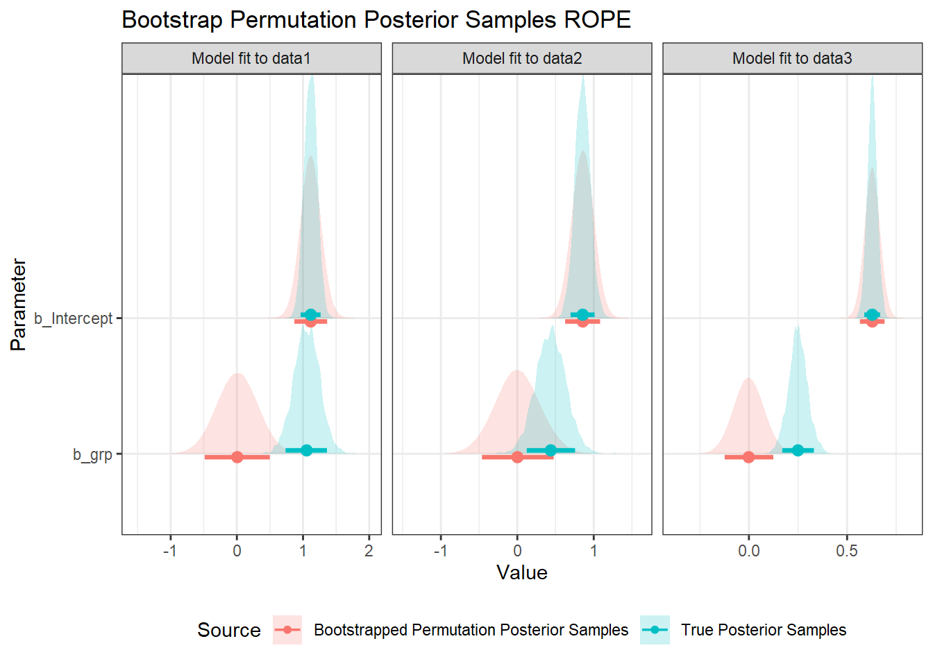

The intercept is unsurprisingly unchanged, as the overall mean is exactly the same, and grp is deviation-coded. The estimate for grp from the bootstrapped permutation estimates is always centred on zero, with the spread reflecting variability we could expect under the null hypothesis for the sampled observations.

From this analysis, we might make the following decisions on the data:

• data1: Accept the alternate hypothesis: the 89% intervals for the posterior samples and bootstrapped permutation estimates do not overlap.

• data2: Inconclusive: The 89% intervals overlap, but the posterior’s interval does not lie entirely within the bootstrap permutation’s estimates’ interval.

• data3: Accept the alternate hypothesis: the 89% intervals for the posterior samples and bootstrapped permutation estimates do not overlap.

Summary of the Pipeline

The pipeline for analysis involves the following steps:

1. Fit desired Bayesian model to the data

2. Fit new models to a large number of bootstrapped versions of the original data in which the effect of interest has been permuted across observations

3. Get the desired highest density interval for the effect estimates from all of the models fit to bootstrapped permutated data for use as the ROPE

4. Compare the desired credible interval of the posterior distribution to this ROPE to make decisions on hypotheses

Conclusion

In cases when, for whatever reason, a theoretically informed ROPE is unavailable, combining bootstraps and permutations could be one solution for calculating a data-driven ROPE. It’s worth pointing out just how flexible this method is. This method could be applied to any Bayesian model under the sun. You could easily incorporate more fixed effects, random effects, smoothing factors. You could also apply the approach to non-linear and multivariate models or models with hierarchical structures.

It’s also worth mentioning that the ROPEs do not have to come from the same dataset you use to test the hypotheses. You could, for example, use prior data to calculate a data-driven ROPE before you start collecting data.

Bonus - Just Use Estimates

Above, I collapse across all the models fit to bootstrapped, permuted data to get a distribution of posterior samples under the null hypothesis. If this is too computationally intensive (as it can be a lot of data), an alternative could be to sample random subsets from the posterior, or to just use the best estimate of each model. Here is a version of the plot above, using the 89% confidence interval of the bootstrap-permutation models’ estimates as the ROPE, rather than the samples:

res_est <- map_df(1:3, function(data_nr) {
  # get the true data's posterior samples
  post_long <- posterior_samples(Ms[[data_nr]]) %>%
    pivot_longer(c(b_Intercept, b_grp), names_to="param", values_to="value") %>%
    mutate(src = "True Posterior Samples")

  # get the estimates from each bootstrapped permuted data
  bsp_est <- bsp_Ms[[data_nr]] %>%
    map_df(function(m_i) {
      fixef(m_i) %>%
        as_tibble(rownames="param")
    }) %>%
    rename(value=Estimate) %>%
    mutate(
      src="Bootstrapped Permutation Estimates",
      param=sprintf("b_%s", param)
    )
  
  # combine into one dataframe
  bind_rows(post_long, bsp_est) %>%
    mutate(df=sprintf("Model fit to data%g", data_nr))
})

res_est %>%
  ggplot(aes(value, param, fill=src, colour=src)) +
  geom_density_ridges(alpha=0.2, colour=NA) +
  stat_pointinterval(.width=0.89, position=position_dodgev(height = 0.1)) +
  labs(
    x = "Value", y = "Parameter", fill="Source", colour="Source",
    title="Bootstrap Permutation Posterior Estimates ROPE"
  ) +
  facet_wrap(vars(df), scales="free_x") +
  theme(legend.position = "bottom")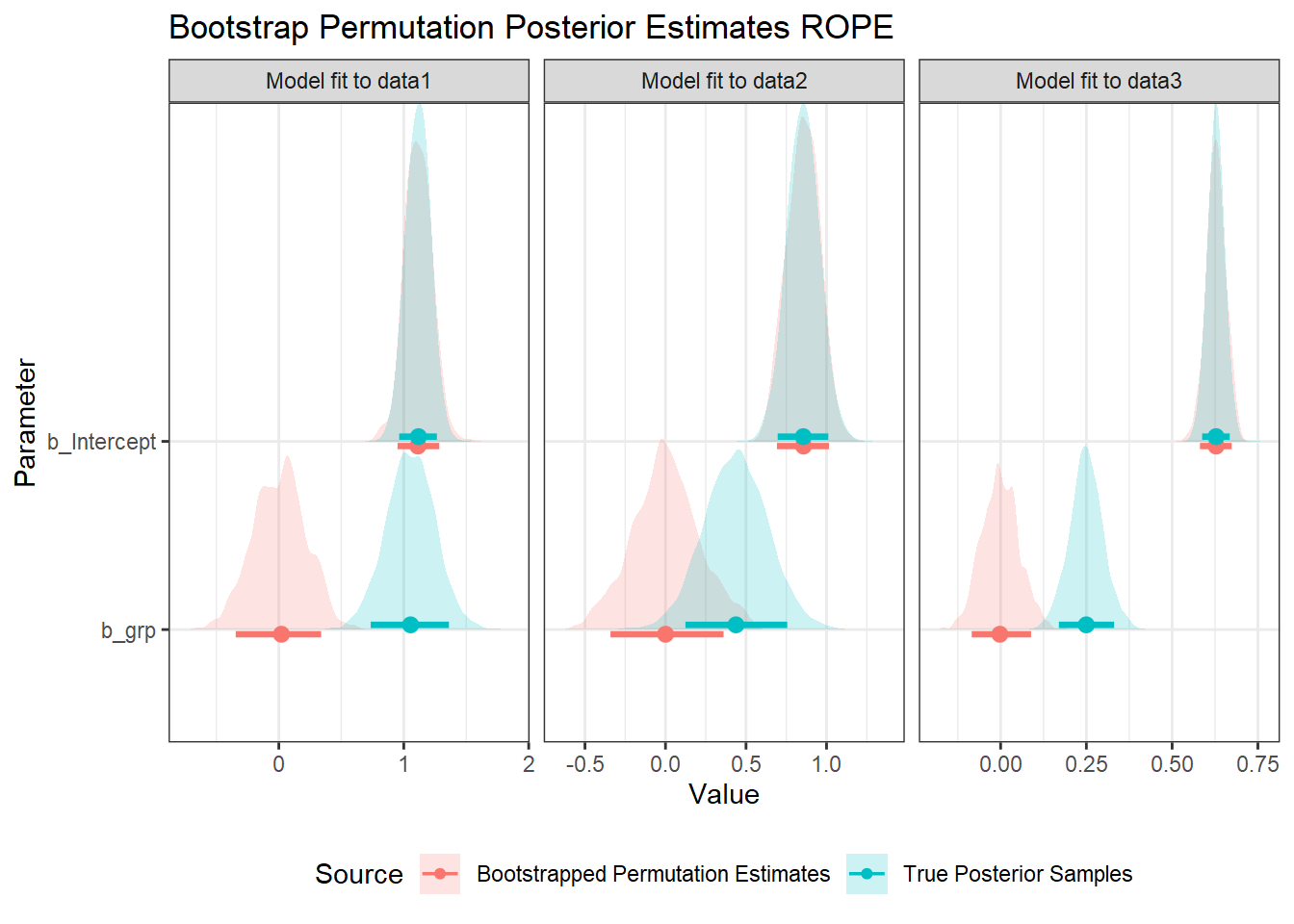

Note that the ROPE using the models’ estimates is somewhat less conservative, however, with similar spread to the original data’s posterior. If we wanted to simulate the spread of the posterior, we could also noise-inflate this with a normal distribution, with a spread equal to that of the collapsed posterior distribution. The distributions are also less regular, though they smooth out if more models are fit (there are only 500 observations here).