Item-Wise and Distribution-Wise Matching
July 6, 2020 - 8 minutes
When designing stimuli, researchers are often very vague about how they created their stimuli. Here, I introduce two reproducible approaches: item-wise and distribution-wise matching.
R LexOPS stimuli psycholinguistics“Words were controlled between conditions for frequency and length (all F values < 1).”
How many times have you read a paper with a sentence like this in the Materials section? This is a problem because of:
Statistical reasons: They’re assuming all kinds of things about their variables (e.g. that they’re all normally distributed), and more importantly, interpreting a non-significant p-value as evidence for equivalence. A small but “non-significant” difference in a confounding variable could have a very real and noticeable effect on an outcome when you repeat the same stimuli across hundreds of trials and many subjects.
Ambiguity: What corpus of frequency did they use? Exactly how well controlled are the stimuli? No one can read that sentence and exactly reproduce the process you used to create your stimuli.
So what’s the solution? Well, we could check distributional assumptions and use an equivalence test to show evidence of practical equivalence (see Lakens et al., 2018 for a good tutorial), but then we’re still acting like the stimuli just randomly appeared on our doorstep one day, and we decided on a whim to use them in a study.
The truth is we have complete control over what stimuli we use. Instead, then, it makes sense to focus on precisely specifying how our stimuli are matched. There are two main approaches to controlling for confounding variables in this way, when you are sampling from a finite number of possible stimuli (as is the case for e.g. a database of words or faces).
item-wise matching, in which each item from condition a is matched in terms of the confounding variables within a certain tolerance to an item in condition b
distribution-wise matching, in which the overall distributions of confounding variables between conditions a and b are matched.
In this post, I’ll show example implementations of these approaches in R, and briefly discuss their differences. In case you want to follow along at home, here’s the code to simulate the data I’ll be using. This dataframe is an imaginary database of face images for a study we’ll imagine we’re running on face perception:
library(tidyverse)
n_stim <- 1000
set.seed(1)

face_stim <- tibble(
  stim_id = sprintf("face_%g", 1:n_stim),
  gender = as.factor(sample(c("m", "f"), size=n_stim, replace=TRUE)),
  age = sample(18:60, size=n_stim, replace=TRUE),
  face_width = rnorm(n_stim, 65, 2.5)
) %>%
  mutate(face_width = if_else(gender=="f", face_width-2.5, face_width))
Item-Wise Matching
Something I’ve worked on quite a bit for the last couple of years has been the R package, LexOPS. If you’re interested in finding out more, there’s an online walkthrough for the package. Long story short, it makes it easy to create lists of matched items for experiments. For example, imagine we have a database of faces that looks like this:
face_stim
## # A tibble: 1,000 × 4
##    stim_id gender   age face_width
##    <chr>   <fct>  <int>      <dbl>
##  1 face_1  m         53       67.6
##  2 face_2  f         37       68.2
##  3 face_3  m         48       68.3
##  4 face_4  m         30       62.8
##  5 face_5  f         20       61.2
##  6 face_6  m         57       66.5
##  7 face_7  m         41       65.0
##  8 face_8  m         46       65.7
##  9 face_9  f         27       59.2
## 10 face_10 f         30       61.4
## # ℹ 990 more rows
If we want to generate 50 matched pairs of male and female faces with similar ages and face widths, we could do this in LexOPS like so:
library(LexOPS)

gen_faces <- face_stim %>%
  set_options(id_col = "stim_id") %>%
  split_by(gender, "f" ~ "m") %>%
  control_for(age, -1:1) %>%
  control_for(face_width, -0.5:0.5) %>%
  generate(50)
This matches faces item-wise, so that male face i is comparable to female face i. Here are the first five matched pairs:
head(gen_faces, 5)
##   item_nr       A1       A2 match_null
## 1       1 face_474 face_375         A1
## 2       2 face_272 face_514         A2
## 3       3 face_836 face_778         A1
## 4       4 face_573 face_264         A1
## 5       5 face_819 face_729         A2
To visualise the generated stimuli, we can plot each face’s location in the age and face width distributions, with lines connecting male and female faces which are matched:
plot_design(gen_faces, include="controls")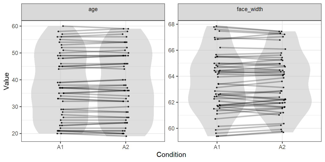
We could use the stimulus lists in gen_faces, and be pretty certain that we have items in both condition which are comparable in the variables of age and face width. In our paper, we could say:
“Stimuli consisted of 50 matched pairs of male and female faces, matched in terms of age (within ±1 year) and face width (within ±0.5 cm), generated with LexOPS (Taylor et al., 2020). The code used to generate the stimuli is available at osf.io/osflinkhere.”
Item-wise matching is useful when you want to ensure items are as directly comparable as possible. The similarity in distributions is a necessary by-product, with the degree of distributional similarity for a given variable depending on how closely items are matched on it, and how many items are used.
Distribution-Wise Matching
An alternative approach is to just maximise the similarity between the groups’ distributions. The approach I’m going to suggest here just maximises distributional overlap of two random samples of the dataset. To do this, I’m going to use the overlapping package (Pastore & Calcagni, 2019) to get an estimate of empirical distributional overlap. You could also match distributional parameters, for example matching the mean (\(\mu\)) and standard deviation (\(\sigma\)) of a normal distribution, but these require strict assumptions which are often inappropriate.
For 20000 iterations (this will take a while), here we take a random sample of 50 male faces, and 50 female faces, and record the degree of distributional overlap (using purrr’s map_df() function to record the output in a dataframe):
library(overlapping)

seed_results <- map_df(1:20000, function(seed_i) {
  # get the sample of 50 male and 50 female faces
  set.seed(seed_i)
  sample_i <- face_stim %>%
    group_by(gender) %>%
    slice_sample(n = 50)
  # get the male-female overlap for age
  ov_age <- overlap(list(
    filter(sample_i, gender=="f") %>% pull(age),
    filter(sample_i, gender=="m") %>% pull(age)
  )) %>%
    with(OV)
  # get the male-female overlap for face width
  ov_face_width <- overlap(list(
    filter(sample_i, gender=="f") %>% pull(face_width),
    filter(sample_i, gender=="m") %>% pull(face_width)
  )) %>%
    with(OV)
  # return the result
  tibble(
    seed = seed_i,
    ov_age = ov_age,
    ov_face_width = ov_face_width
  )
})
Now we have the overlap indices for males’ and females’ distributions in the two variables, for each of the 20000 seeds.
seed_results
## # A tibble: 20,000 × 3
##     seed ov_age ov_face_width
##    <int>  <dbl>         <dbl>
##  1     1  0.823         0.412
##  2     2  0.811         0.419
##  3     3  0.810         0.595
##  4     4  0.810         0.483
##  5     5  0.671         0.545
##  6     6  0.846         0.525
##  7     7  0.825         0.360
##  8     8  0.787         0.453
##  9     9  0.680         0.531
## 10    10  0.794         0.388
## # ℹ 19,990 more rows
We really want a single value to optimise by. An easy solution is to just take the average. This can also be weighted if it’s more important for some variables to be matched than others (e.g. if you think age is a larger confound than face width).
seed_results <- mutate(seed_results, ov_avg = (ov_age + ov_face_width)/2)We can recreate the simulated samples using the desired seeds. This is how similar the male and female distributions are for the best random sample:
best_seed <- seed_results %>%
  filter(ov_avg == max(ov_avg)) %>%
  pull(seed)

set.seed(best_seed)
best_sample <- face_stim %>%
  group_by(gender) %>%
  slice_sample(n = 50)

best_sample %>%
  pivot_longer(cols = c(age, face_width), names_to="Parameter", values_to="Value") %>%
  ggplot(aes(Value, fill=gender)) +
  geom_density(alpha=0.5) +
  facet_wrap(vars(Parameter), scales="free")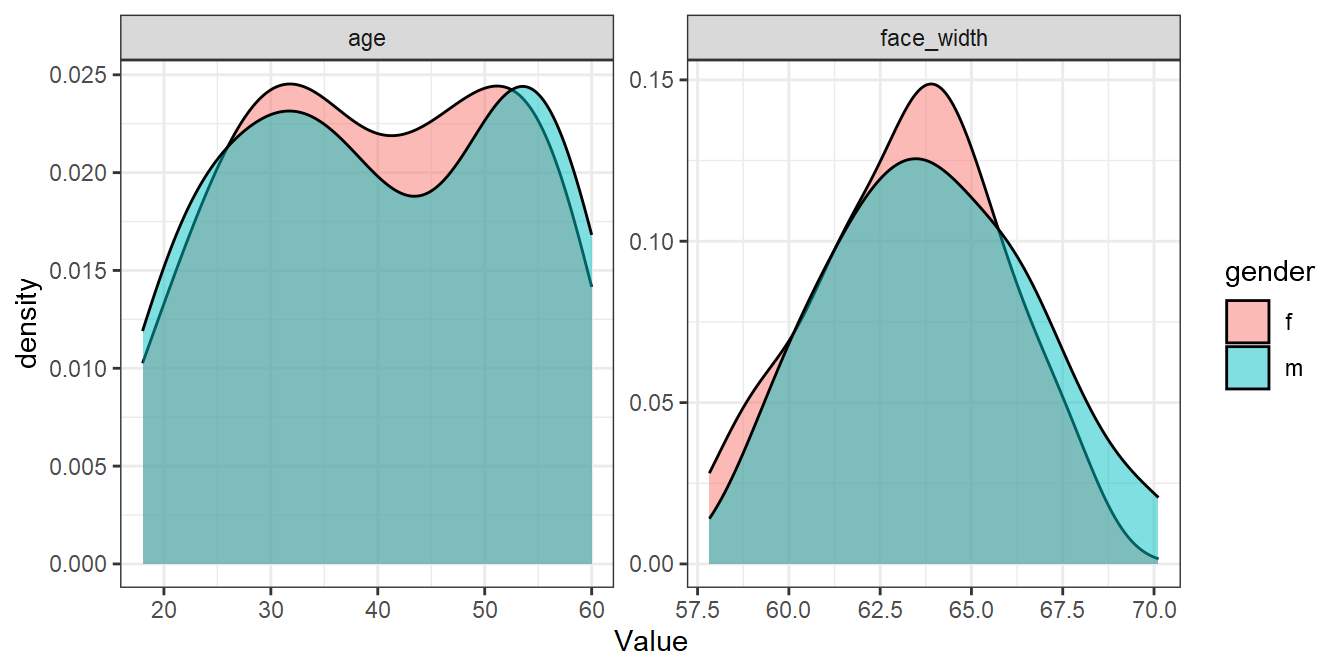
For comparison, here’s the worst sample:
worst_seed <- seed_results %>%
  filter(ov_avg == min(ov_avg)) %>%
  pull(seed)

set.seed(worst_seed)
worst_sample <- face_stim %>%
  group_by(gender) %>%
  slice_sample(n = 50)

worst_sample %>%
  pivot_longer(cols = c(age, face_width), names_to="Parameter", values_to="Value") %>%
  ggplot(aes(Value, fill=gender)) +
  geom_density(alpha=0.5) +
  facet_wrap(vars(Parameter), scales="free")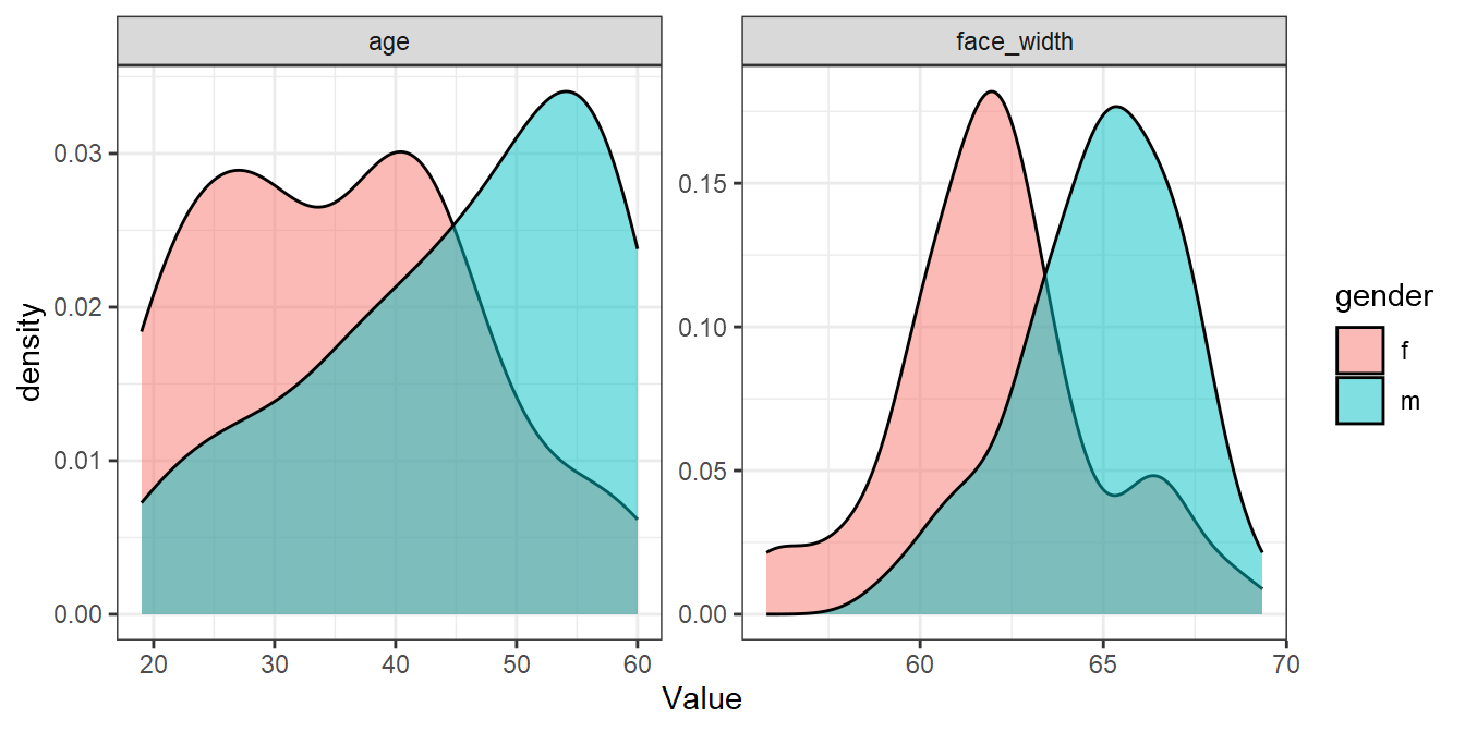
Not bad considering! We could use the stimuli in best_sample for an experiment and be fairly confident that there are no large differences in age or face width. In our paper, we could report that:
“We selected a stimulus set which maximised distributional overlap, measured with the assumption-free overlap index (Pastore & Calcagni, 2019), from 20000 randomly generated lists of 50 male and 50 female faces. The selected stimulus set resulted in an overlap index of 0.91 for age, and 0.84 for face width. The code used to generate the stimuli is available at osf.io/osflinkhere.”
It’s worth mentioning that you’ll get nicer matches as you run more iterations. The number of iterations you need to identify a suitable set will depend on things like the size of your stimulus pool and the number of variables you are trying to match. The more iterations you run the algorithm for, the better a result you’ll find. Here’s a plot demonstrating that for the iterations I ran above:
seed_results %>%
  mutate(
    age = cummax(ov_age),
    face_width = cummax(ov_face_width),
    average = cummax(ov_avg)
  ) %>%
  pivot_longer(c(age, face_width, average), names_to="dist", values_to="best_val") %>%
  ggplot(aes(seed, best_val, colour=dist, group=dist)) +
  geom_line() +
  labs(x = "Iteration", y = "Best Overlap Value", colour = "Distribution")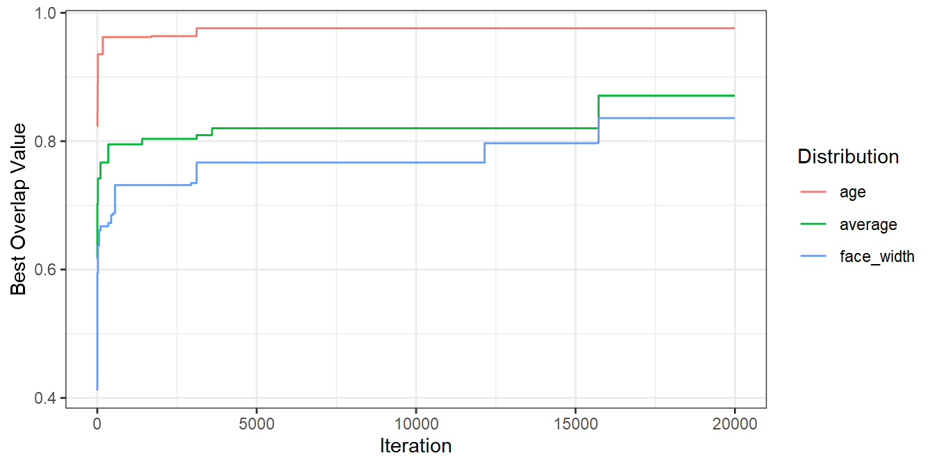
Summary
Distribution-wise and item-wise matching are two different ways to controlling your stimuli. Item-wise matching has the advantage of giving sets of items which are directly comparable on all dimensions. On the other hand, the distribution-wise approach is very flexible - the pipeline can easily be altered to optimise parameters other than overlap, for example, or to maximise the similarity to the population distribution (if known) if you’re especially interested in generalisability. There’s also no reason why you can’t use a combination of the methods, like controlling for confounds between levels of a predictor with item-wise matching, and implementing a counterbalanced design with distribution-wise matching.
These methods are reproducible! This means we can share the code and resulting stimuli along with papers, so other researchers can easily see what we did, and try to replicate effects or alter the pipelines for their own purposes, for instance adding additional controls.
In other words: be specific, be reproducible, share your stimuli, and share your code!
More!
If you liked this post, you might also be interested in a workshop hosted at SIPS 2021: https://jackedtaylor.github.io/SIPS2021/