01 - Item-Wise Matching
When you match item-wise, you’re finding items in each condition which are directly comparable across control variables. In this example, I’ll show a simple item-wise example controlling for one variable.
Setup
Load Packages
library(tidyverse)
library(LexOPS)  # package with functions for item-wise matching
Import the Data
stim_pool <- read_csv("stim_pool.csv")Item-Wise Matching with LexOPS
Step 1: Find Matches
Let’s create a list of 100 young and 100 old faces, matched on face width within ±0.5 pixels. We can do this all in one go with LexOPS.
- Use
set_options()to tell LexOPS which column contains the stimulus IDs - Use
split_by()to specify the conditions - Use
control_for()to specify the control variable - Use
generate()to find 100 matches, with a seed for reproducibility
stim <- stim_pool %>%
  set_options(id_col = "stim_id") %>%
  split_by(age, 1:28 ~ 50:100) %>%
  control_for(face_width, -0.5:0.5) %>%
  generate(n=100, seed=42)
## Generated 5/100 (5%). 5 total iterations, 1.00 success rate.
Generated 10/100 (10%). 10 total iterations, 1.00 success rate.
Generated 15/100 (15%). 15 total iterations, 1.00 success rate.
Generated 20/100 (20%). 20 total iterations, 1.00 success rate.
Generated 25/100 (25%). 25 total iterations, 1.00 success rate.
Generated 30/100 (30%). 30 total iterations, 1.00 success rate.
Generated 35/100 (35%). 35 total iterations, 1.00 success rate.
Generated 40/100 (40%). 40 total iterations, 1.00 success rate.
Generated 45/100 (45%). 45 total iterations, 1.00 success rate.
Generated 50/100 (50%). 50 total iterations, 1.00 success rate.
Generated 55/100 (55%). 55 total iterations, 1.00 success rate.
Generated 60/100 (60%). 60 total iterations, 1.00 success rate.
Generated 65/100 (65%). 65 total iterations, 1.00 success rate.
Generated 70/100 (70%). 70 total iterations, 1.00 success rate.
Generated 75/100 (75%). 75 total iterations, 1.00 success rate.
Generated 80/100 (80%). 80 total iterations, 1.00 success rate.
Generated 85/100 (85%). 85 total iterations, 1.00 success rate.
Generated 90/100 (90%). 90 total iterations, 1.00 success rate.
Generated 95/100 (95%). 95 total iterations, 1.00 success rate.
Generated 100/100 (100%). 100 total iterations, 1.00 success rate.This gives us a list of matched pairs of young and old faces. Each row has a young face A1, and old face A2, and match_null (usually only relevant for designs with >2 conditions - see 04 - Setting the Match Null):
stim## # A tibble: 100 x 4
## item_nr A1 A2 match_null
## <int> <chr> <chr> <chr>
## 1 1 face_4884 face_4197 A1
## 2 2 face_4022 face_1960 A1
## 3 3 face_1307 face_3654 A2
## 4 4 face_2516 face_163 A2
## 5 5 face_117 face_3006 A1
## 6 6 face_2901 face_913 A1
## 7 7 face_175 face_2151 A2
## 8 8 face_3958 face_2218 A1
## 9 9 face_2983 face_3459 A1
## 10 10 face_2139 face_3470 A1
## # ... with 90 more rowsStep 2: Check Stimuli
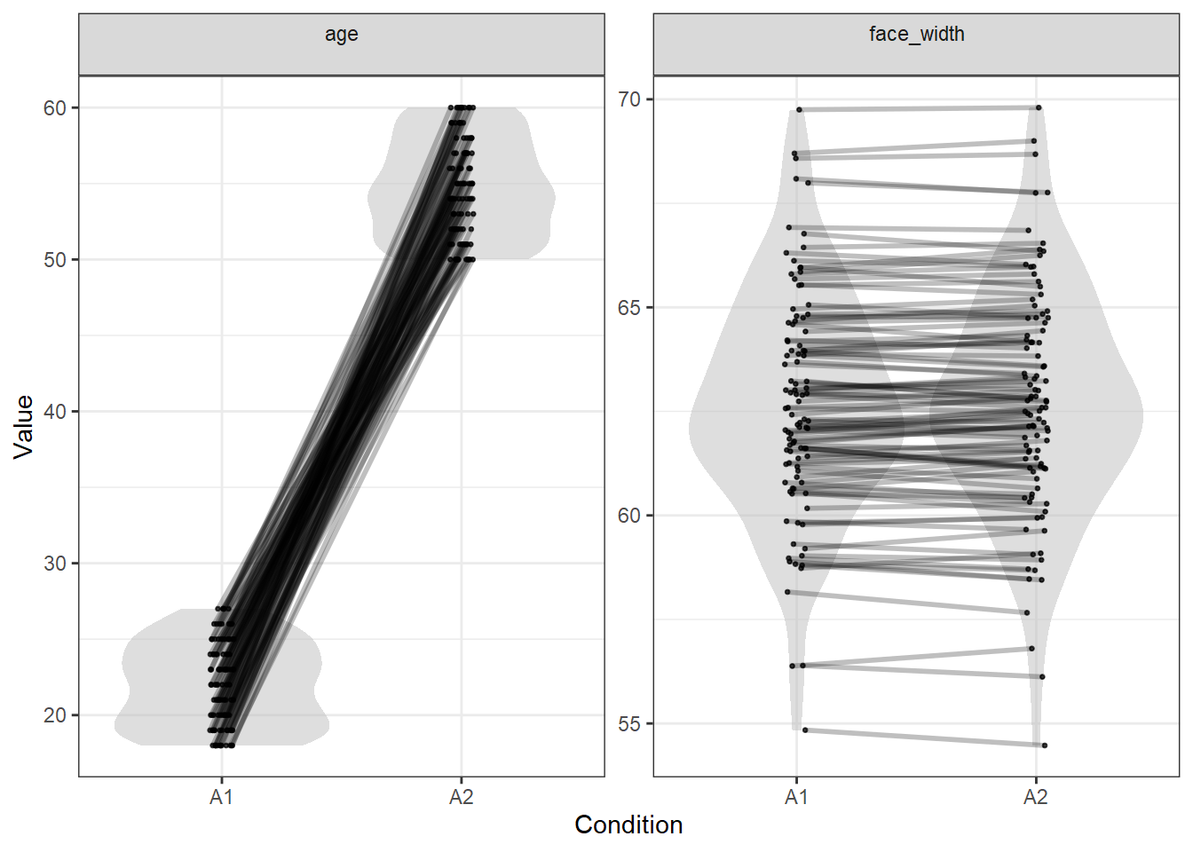
We can quickly check how well our stimuli are matched with the plot_design() function.
plot_design(stim)
This shows the expected result, where:
- Condition A1 is all young faces, while condition A2 is all old faces
- Condition A1 and A2 are matched pairwise for face width - note that this also results in very similar distributions