03 - Multiple Control Variables
In this example, let’s match on more than one control variable. We’ll use the same design as in 01 - Maximising Distributional Overlap, but control for three variables simultaneously: face_width, face_length, and task_rt. We’ll match for variables using the Overlapping Index (although we could use other statistics if we wanted).
Setup
Load Packages
library(tidyverse)
library(overlapping)  # contains function for calculating overlap index
Import the Data
stim_pool <- read_csv("stim_pool.csv")Matching Using Multiple Controls
As mentioned, we’ll again create a list of 100 young and 100 old faces. This time, however, we’re matching on face width, face length, and response time on a task (task_rt). If stim_pool is a pool of normed candidate items, you could think of task_rt as an average response time in a face recognition task (in milliseconds).
Step 1: Identify conditions
First, we define our conditions. We’ll use the same conditions as in 01 - Maximising Distributional Overlap.
stim_pool <- mutate(stim_pool, cond = case_when(age<28 ~ "young", age>50 ~ "old"))Step 2: Create a vector of seeds
As before, we’ll create a vector of a large number of random seeds so we can reproduce our stimulus sets. For speed, I’m only running 1000 iterations in this example, but I recommend running much larger numbers of iterations to improve the quality of the match.
set.seed(3101)  # comment this line out (put # at the start of the line) to get a different result to mine
n_iter <- 1000
seeds <- sample(1:.Machine$integer.max, n_iter)
Step 3: Identify the Control Variables
We’ll create a vector of the column names for the variables we want to control for. We’ll use this to loop over the control variables.
control_vars <- c("face_width", "face_length", "task_rt")Step 4: Simulate a large number of samples
As before, we want to simulate a large number of random samples. This time, however, we’re recording distributional overlap on three different control variables. To do this, we can just use a nested sapply() loop.
res <- map_df(seeds, function(seed_i) {
  # set the seed, so we can recreate any sample later
  set.seed(seed_i)

  sample <- stim_pool %>%
    # only keep observations from conditions we are interested in (remove faces from ages 29 to 49)
    filter(cond %in% c("young", "old")) %>%
    # for each condition, randomly select 100 items
    group_by(cond) %>%
    slice_sample(n = 100)

  # for each control variable, record the overlap between the two conditions
  control_ov <- sapply(control_vars, function(var_i) {
    # get the values for this control variable for the young condition
    var_i_young <-  sample %>%
      filter(cond == "young") %>%
      pull(!!var_i)

    # get the values for this control variable for the old condition
    var_i_old <-  sample %>%
      filter(cond == "old") %>%
      pull(!!var_i)

    # get the degree of overlap on the control variable between the two samples
    ov_results <- overlapping::overlap(list(var_i_young, var_i_old))

    # extract the actual value for the degree of overlap
    ov_results$OV
  })

  # return a dataframe with the overlap for the three control variables
  tibble(seed = seed_i, control = control_vars, ov = control_ov)
})
Step 5: Calculate overall overlap
Now that we’re controlling for multiple variables, we want to make sure we’re matching overall overlap, rather than overlap for each variable individually. To do this, we can just calculate the average overlap for each seed:
res_summ <- res %>%
  group_by(seed) %>%
  summarise(mean_ov = mean(ov))
Step 6: Check the results
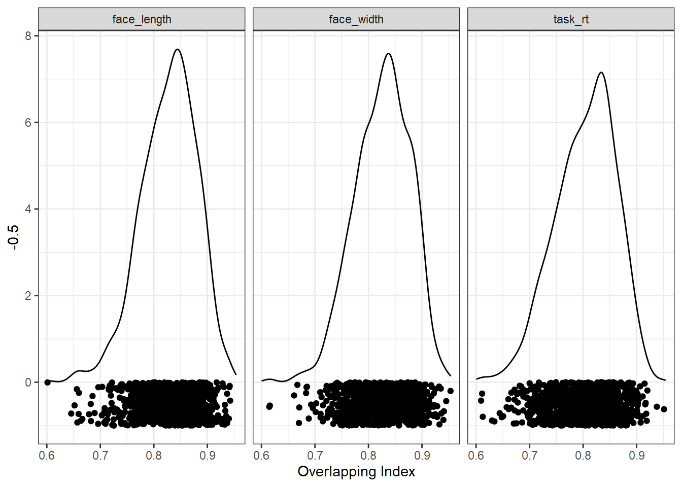
We can now look at the distribution of overlapping index values from all the random samples. The closer to 1, the better the overlap. Here are the distributions for each control variable separately:
ggplot(res, aes(ov)) +
  geom_density() +
  geom_point(aes(y = -0.5), position = position_jitter(height=0.5)) +
  xlab("Overlapping Index") +
  facet_wrap(vars(control))
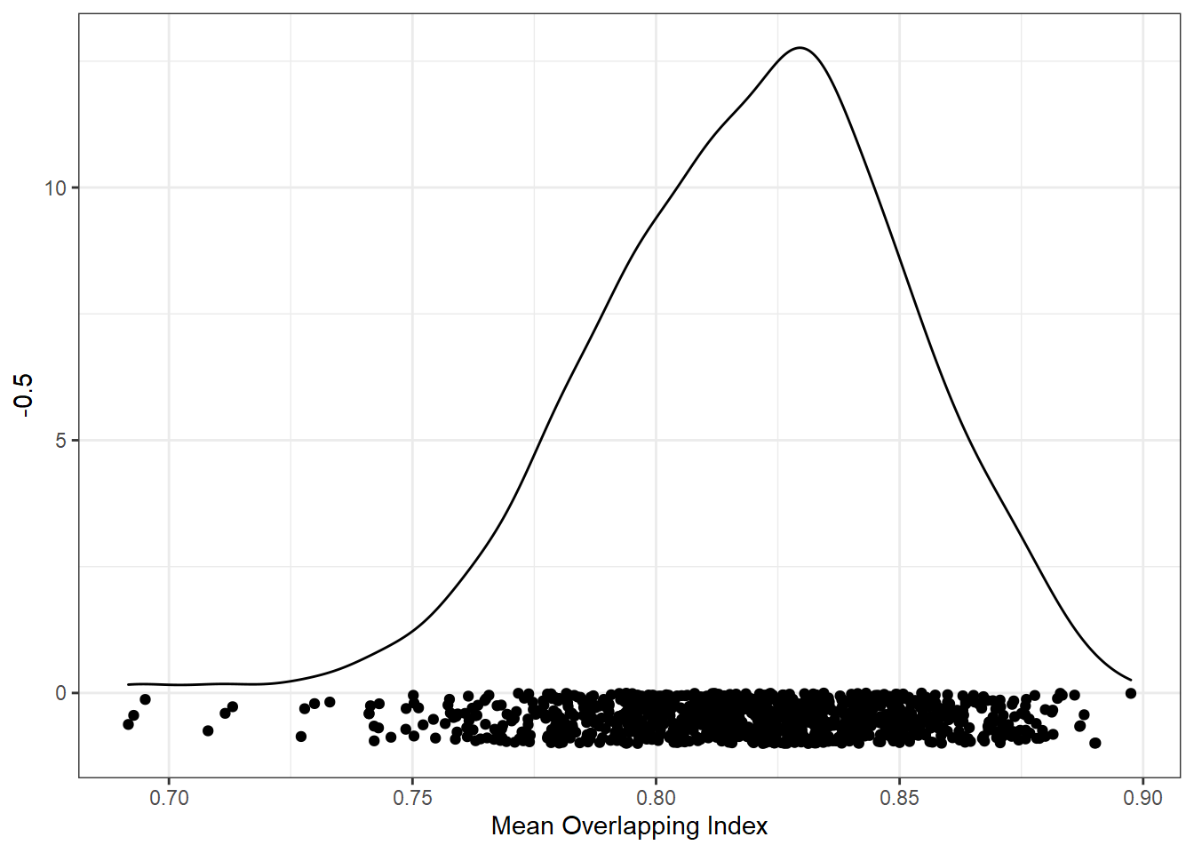
But remember, we want to match conditions using overlap in all variables. Here is the distribution of the mean of the overlap index values.
ggplot(res_summ, aes(mean_ov)) +
  geom_density() +
  geom_point(aes(y = -0.5), position = position_jitter(height=0.5)) +
  xlab("Mean Overlapping Index")
Step 7: Find the best stimulus set
We can now sort the results by mean overlapping index (descendingly) to order them by how well-matched the conditions are.
res_sorted <- arrange(res_summ, desc(mean_ov))

res_sorted
## # A tibble: 1,000 x 2
## seed mean_ov
## <int> <dbl>
## 1 661908874 0.897
## 2 438788215 0.890
## 3 1184616802 0.890
## 4 1275019465 0.888
## 5 330925025 0.887
## 6 459083624 0.887
## 7 928881234 0.886
## 8 568423763 0.883
## 9 1826604304 0.883
## 10 1156924132 0.882
## # ... with 990 more rowsNow we can just extract the best seed as that which has the highest overlapping index.
# sort by distance ascendingly, so the best seed is at the top, and extract it
best_seed <- res_sorted %>%
  pull(seed) %>%
  first()

best_seed
## [1] 661908874Step 8: Recreate the best stimulus set
Now we know that 661908874 is the best seed, we can use that seed to recreate the stimulus set. This code needs to be identical to our simulation code to ensure we recreate the exact same stimulus set.
set.seed(best_seed)

best_stim <- stim_pool %>%
  filter(cond %in% c("young", "old")) %>%
  group_by(cond) %>%
  slice_sample(n = 100)
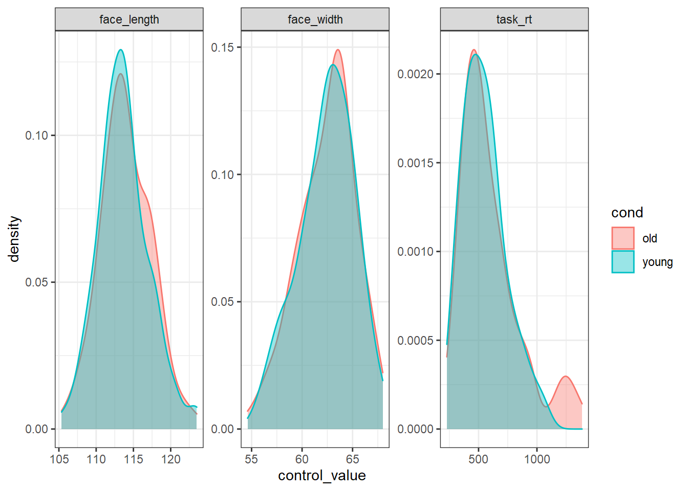
To prove that the stimuli are well-matched, here is what the distribution of each control variable looks like in each condition:
best_stim %>%
  pivot_longer(all_of(control_vars), names_to="control", values_to="control_value") %>%
  ggplot(aes(control_value, colour=cond, fill=cond)) +
  geom_density(alpha=0.4) +
  facet_wrap(vars(control), scales="free")
We could use the faces in best_stim for our experiment, and be fairly sure that we’ve controlled for face width.
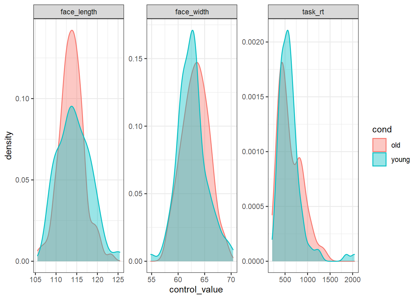
For comparison, here is what the worst stimulus set looks like:
# sort ascendingly (smallest overlap first), and extract the top seed
worst_seed <- res_sorted %>%
  arrange(mean_ov) %>%
  pull(seed) %>%
  first()

set.seed(worst_seed)

# recreate the worst stimulus set
worst_stim <- stim_pool %>%
  filter(cond %in% c("young", "old")) %>%
  group_by(cond) %>%
  slice_sample(n = 100)

worst_stim %>%
  pivot_longer(all_of(control_vars), names_to="control", values_to="control_value") %>%
  ggplot(aes(control_value, colour=cond, fill=cond)) +
  geom_density(alpha=0.4) +
  facet_wrap(vars(control), scales="free")